When applying an arithmetic conversion some of the resulting values may be indefinite. Epina ImageLab distinguishes between "hard errors" and "soft errors". Hard errors can be recognized before the transformation starts. Those errors are reported immediately and the conversion cannot be started. Soft errors emerge during the actual calculations. They are counted and reported to the user at the end of the conversion process. Each cell of the data cube which gives rise to a soft error is filled whenever possible by a reasonable value (which results from the consideration of the mathematical limit of the particular transformation) or else by the indefinite substitute value (which is, by default, set to -1, but can be adjusted in the preferences dialog).
The following table provides a list of available conversions (x represents the spectral data):
| Transformation |
Explanation/Remarks |
| Transmission to Absorbance | Converts the transmission Trm to the absorbance Abs using the equation Abs = -lg(Trm). The data must be greater than zero. |
| % Transmission to Absorbance | Converts the percent transmission %Trm to the absorbance Abs using the equation Abs = 2-lg(Trm). The data must be greater than zero. |
| Absorbance to Transmission | Converts the absorbance Abs to the transmission Trm using the equation %Trm = 10(-Abs). The data must be greater than zero. |
| Absorbance to %Transmission | Converts the absorbance Abs to percent transmission %Trm using the equation %Trm = 10(2-Abs). The data must be greater than zero. |
| Add (B*x + A) | Scales the data by a factor of B and adds the constant A. |
| Multiply (x * A) | Multiplies the data by the constant A |
| Divide (x / A) | Divides the data by the constant A; A must not be zero |
| Inverse (A / x) | Calculates the inverse of the data times A. If the data is zero it is replaced by the indefinite value specified in the preferences dialog. |
| Power (x ^ A) | Raises the data to the power A. If the parameter A is a fractional number the data has to be greater than zero. |
| Root (x ^ (1/A)) | Draws the root of base A. The parameter A must be greater than zero. |
| Fraction (frac(x*A)) | Calculates the fractional part after multiplying the data by A. Please note that this is equivalent to the modulo function for integer numbers. |
| Logarithm (base A) | Calculates the logarithm of base A. The parameter A must be greater than zero. |
| Exponential (A^x) | Calculates the exponential with base A. The parameter A must be greater than zero. |
| Replacement (A<--B) | Replaces all values equal to parameter A by the value of parameter B. Please note that the comparison of data values to the parameter A might fail due to round-off errors. It is thus recommended to use the replacement option only for integer numbers. |
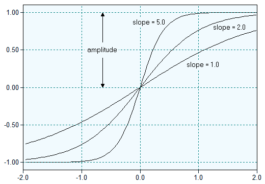
| Sigmoid (amplitude A, slope B) | Applies the sigmoid function (see the diagram below for details). |
| Add Noise (A = homo, B = hetero) | Adds normally distributed noise. The parameter A controls the amount of homoscedastic noise, the parameter B the amount of heteroscedastic noise. Each data value x is transformed by the following equation: x := x + nse*(ParA + ParB*x), with nse being a random value drawn from a standard normal distribution (µ = 0, s = 1). |
The following diagram shows the transfer characteristic of the sigmoid function for an amplitude of 1.0 and various slopes:
 Preprocessing


 Preprocessing > Predefined Arithmetic Conversions