Home  Tools LIBS Tool LIBS Tool Tools LIBS Tool LIBS Tool |
|||||||||||||||||||||||
See also: Import: ASI LIBS (Clarity)
 |
|||||||||||||||||||||||
  |
|||||||||||||||||||||||
LIBS Tool |
|||||||||||||||||||||||
|
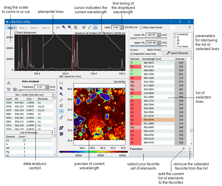
The LIBS tool is a tool specifically taylored to the analysis of LIBS data. It consists of the following principal sections:
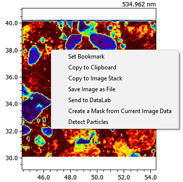
Preview ImageThe preview image allows you to display an image of a particular wavelength and use this image for further actions. All those actions can be performed by right clicking the image, which opens the following context menu:
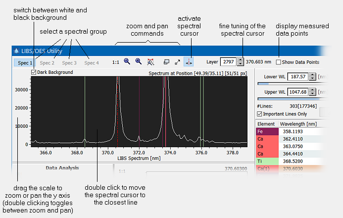
Spectral diagramThe spectral diagram displays the spectrum at the location cursor. The options of this diagram are described in the following figure:
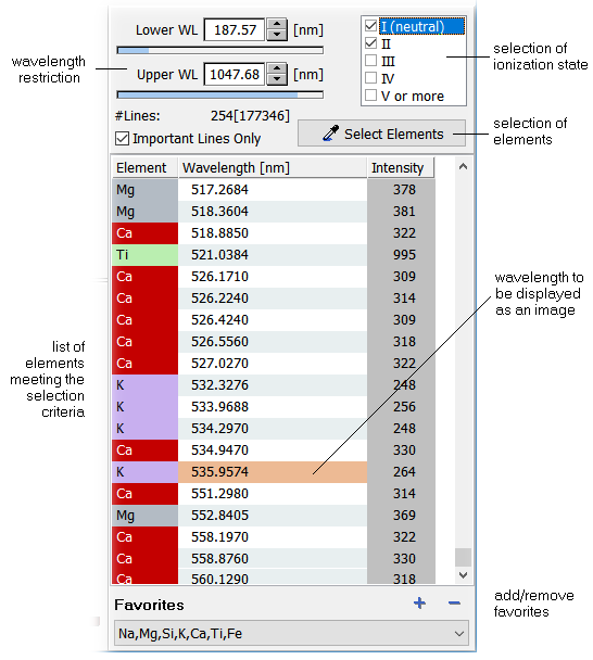
Selection of elemental linesThe database of elemental emission lines contains about 180000 lines in the range between 100 and 1200 nm. You can narrow down the display of lines by various restriction parameters: (1) wavelength restriction, (2) selection of elements, (3) selection of ionization state and (4) important lines only. Further, you can store the current selection of elements and the restrictions as a favorite by clicking the "plus" button.
Data analysisThe data analysis section provides three tools which support you in the analysis of spectral lines:
|
|||||||||||||||||||||||
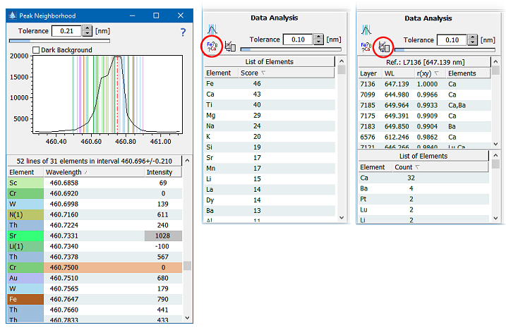
 Spectral neighborhood: clicking this button opens another window (left in the figure below) which shows the signal and all elemental lines around the spectral cursor. More important elemental lines are indicated by a gray background in the intensity column. Double-clicking an element adds/removes it to/from the selection of elements.
 Matching spectral lines: this tries to find those elements whose lines match the measured spectrum. The result is displayed as a sorted list showing the best matching elements and their correspoding scores. Scores greater above 25 provide a strong indication that the respective element is contained in the spectrum, scores below 15 are more or less random findings. Please note that the elemental analysis is always applied to the currently visible spectrum. Thus moving the location cursor in the image allows you to analyse different regions of the image. Further you can analyse the mean spectrum of a region by using the lasso tool.
 Correlating layers: this analysis allows you to find layers which are most similar to the currently displayed one. The idea behind is that similar images must come from common elemental lines. Thus it is possible to assign an element to a particular spectral line by counting the matches of the layers which are similar to lines contained in the spectra database. The results are shown in the right most part of the figure below. In this case calcium is the most prominent element which indicates that the currently selected layer is due to a calcium line in the LIBS spectrum.